Interactive online version:
![]()
Getting started
This tutorial introduces basic concepts and practices of PAX.
[1]:
import jax
import jax.numpy as jnp
import pax
import matplotlib.pyplot as plt
from absl import logging
[2]:
logging.set_verbosity(logging.FATAL)
plt.rcParams["figure.figsize"] = (3, 2)
To demonstrate the basics of pax.Module, we will define a simple Linear module with an additional forward pass counter.
[3]:
class Linear(pax.Module):
    def __init__(self):
        super().__init__()
        self.weight = jnp.array(1.0)
        self.bias = jnp.array(0.0)
        self.counter = jnp.array(0)

    parameters = pax.parameters_method("weight", "bias")

    def __call__(self, x: jnp.ndarray) -> jnp.ndarray:
        self.counter = self.counter + 1
        return self.weight * x + self.bias

    def __repr__(self):
        return f"Linear(weight={self.weight:.3f}, bias={self.bias:.3f}, counter={self.counter})"
The function call pax.parameters_method("weight", "bias") returns a parameters method that considers weight and bias as trainable parameters.
[4]:
net = Linear()
print(net)
Linear(weight=1.000, bias=0.000, counter=0)
Next, we will create a toy dataset for training purposes.
[5]:
def create_data(a=-3.0, b=1.5):
    x = jax.random.uniform(pax.next_rng_key(), (128, 1))
    noise = jax.random.normal(pax.next_rng_key(), x.shape) * 0.2
    y = a * x + b + noise
    return x, y
[6]:
pax.seed_rng_key(42)
x, y = create_data()
PAX keeps a global random key for each thread. We use pax.seed_rng_key(42) to seed that global random key. The function pax.next_rng_key() returns a random key and also renews the global random key.
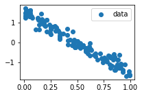
[7]:
def plot_data(x, y):
    plt.scatter(x, y, label="data")
    plt.legend()
    plt.show()
[8]:
plot_data(x, y)
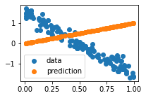
OK, let’s plot the initial predictions of our Linear model.
[9]:
def plot_prediction(x, y, y_hat):
    plt.scatter(x, y, label="data")
    plt.scatter(x, y_hat, label="prediction")
    plt.legend()
[10]:
y_hat = net(x)
plot_prediction(x, y, y_hat)
print(net)
---------------------------------------------------------------------------
ValueError                                Traceback (most recent call last)
<ipython-input-10-236420d1cd7e> in <module>
----> 1 y_hat = net(x)
      2 plot_prediction(x, y, y_hat)
      3 print(net)

<ipython-input-3-26b95aa36ade> in __call__(self, x)
     10
     11     def __call__(self, x: jnp.ndarray) -> jnp.ndarray:
---> 12         self.counter = self.counter + 1
     13         return self.weight * x + self.bias
     14

/workspaces/pax/pax/_src/core/base.py in __setattr__(self, name, value)
    172     def __setattr__(self, name: str, value: Any) -> None:
    173         """Setting `_pax` attribute is forbidden."""
--> 174         self._assert_mutability()
    175
    176         if name == "_pax":

/workspaces/pax/pax/_src/core/base.py in _assert_mutability(self)
    154     def _assert_mutability(self):
    155         if not is_mutable(self):
--> 156             raise ValueError(
    157                 "Cannot modify a module in immutable mode.\n"
    158                 "Please do this computation inside a function decorated by `pax.pure`."

ValueError: Cannot modify a module in immutable mode.
Please do this computation inside a function decorated by `pax.pure`.
Oops! PAX prevents us to update self.counter. Indeed, PAX modules are immutable by default. The only way to modify a module is to pass it as an argument to a function decorated by pax.pure. Below is a working implementation:
[11]:
@pax.pure
def run(net, x):
    y_hat = net(x)
    return net, y_hat
Note that pax.pure only allows run to access to a copy of its input module. This is PAX’s mechanism to purify a function. As a consequence, any modification on the copy will not affect the original module. Therefore, we have to return the updated net in the output.
[12]:
net, y_hat = run(net, x)
plot_prediction(x, y, y_hat)
print(net)
Linear(weight=1.000, bias=0.000, counter=1)
It is inconvenient that we have to manually create a function and decorate it with pax.pure every time we want to call a module. PAX provides the utility function pax.purecall that does the job for us. Below is a more convenient implementation:
[13]:
net, y_hat = pax.purecall(net, x)
To train our model, we need a loss function. In this case, we will define a mean squared error (MSE) loss function as follows:
[14]:
def mse_loss(model: Linear, x, y):
    model, y_hat = pax.purecall(model, x)
    loss = jnp.mean(jnp.square(y - y_hat))
    return loss, model
It is important that we return the updated model in the output of mse_loss. This is required to make the updated model available outside of the loss function.
Next, we will implement a simple stochastic gradient descent (SGD) optimizer to update trainable parameters of our model.
[15]:
def sgd(params: Linear, gradients: Linear, lr: float = 1e-1):
    updated_params = jax.tree_util.tree_map(lambda p, g: p - lr * g, params, gradients)
    return updated_params
Lastly, we need an update function that represents a single training step.
[16]:
@jax.jit
def update_fn(net: Linear, x, y):
    (loss, net), grads = pax.value_and_grad(mse_loss, has_aux=True)(net, x, y)
    params = net.parameters()
    params = sgd(params, grads)
    net = net.update_parameters(params)
    return net, loss
The function pax.value_and_grad is a thin wrapper of jax.value_and_grad. It computes gradients with respect to trainable parameters of the model. We use it to transform the mse_loss function into a function that returns both (loss, net) and the gradients grads.
Also, net.parameters() returns trainable parameters of the model and net.update_parameters(params) returns a new model with parameters updated.
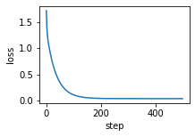
OK, let’s train the model for 500 steps:
[17]:
losses = []

for step in range(500):
    net, loss = update_fn(net, x, y)
    losses.append(loss)

plt.plot(losses)
plt.xlabel("step")
plt.ylabel("loss")
plt.show()
[18]:
net
[18]:
Linear(weight=-3.023, bias=1.496, counter=502)
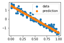
Finally, let’s plot the predictions of our trained model.
[19]:
net, y_hat = pax.purecall(net, x)
plot_prediction(x, y, y_hat)